cdstahl.org

Several previous articles have focused on linear feedback shift registers.  These are very simple circuits which are very often used for generating “maximal” length sequences, which are sequences of all non-zero values of N bits.  “Maximal” does not include the value of 0.  This article discusses some alternative implementations of these simple circuits.

Continue reading →

Previously, I had written an article about how to use non-orthogonal basis vectors for the modeling of sampled data.  Here I show the same idea, but reformulated as a linear regression problem.

Continue reading →

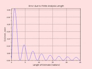
Transforms and projections are often very useful in gaining useful information about a signal.  The Fourier transform is a very common transform that give some information about the frequency content of a signal.  it is not the only possible transform though.

The Problem

In this article, it is assumed that the user will have a samples from a signal with a single frequency.  The sampling rate and input frequency are assumed to be an known, but possibly irrational ratio.  The goal is to determine the magnitude and phase of the single frequency in the input signal.  The length of data for analysis is between one and three cycles of the single input frequency.

There are several ways to solve this problem.  This article focuses on using a projection operator and explains the issue with the Fourier transform in this application.

Fourier Transform

The classic (discrete) Fourier transform has issues with this type of problem.  While it does convert points in time into points in frequency, it only selects N specific frequencies.  Further, these N frequencies will never be exactly correct when the sampling rate is irrationally related to the input frequency.  Finally, increasing sampling rate will also fail to give substantially better results.

The transform essentially comes down to inner products with orthogonal basis vectors based on sines and cosines, as well as a constant term.  It isn’t hard to see how the basis vectors are chosen.  The constant term and one cycle of a sine wave are chosen first.  The cosine is orthogonal to the sine wave over one full cycle.  From this point, only integer multiples of this fundamental frequency will be orthogonal to both the constant term and the sine wave vectors.  This is because the inner product of sine and cosine is non-zero over partial cycles.

As a result of the above “harmonically-related” requirement, the transform will never have a basis vector with exactly the correct frequency for the irrationally-related input.  Without a basis vector at the correct frequency, the transform will approximate the input frequency as the closest basis vector.  The approximation error will then be spread out across the other basis vectors (frequencies).

Finally, oversampling isn’t too useful.  The length of the data, in cycles of the input frequency, doesn’t increase.  Extra points are added to the transform, but they are all added at higher frequencies.

Using Non-Orthogonal Vectors

The issues with the DFT can be aided by using basis vectors that are not orthogonal.  This means the projection or transform is a bit more complicated.  In this case, we will use a projection — we know enough about the input that a transform isn’t needed.  Basically, we can choose basis vectors such that only two would have non-zero coefficients.

For our system, we have:

In the orthonormal (both orthogonal and normalized) case this would be equal to:

Which is very nice, as it simplifies the problem.  We don’t have orthogonal vectors though.  At this point, it’s nice to give some definition to the vectors:

Basically, we are declaring that is the sine and cosine vectors.  These will be useful as the coefficients will be the values of A and B in the input.  But to get these, we have to determine that can be used in the inner products.  For the moment we will make the assumption that is a linear combination of .

From here it is easy enough to create two test cases, eg:

Notice that this gives enough information to determine the inner products.  The end result is four equations, four unknowns.  These can be solved for the values of k.  Finally, a few other test vectors could be used to give some confidence in the solution.

Example

t = 2*pi*pi/32 * [0:80]; % the time vector a few cycles
phi0 = sin(t);
phi1 = cos(t);
f0 = 2*sin(t) + 3*cos(t);
f1 = 3*sin(t) + 2*cos(t);

Now, lets look at the incorrect method and the results:

%% Incorrect
phi0*f0'/81   % 1.0095
phi1*f0'/81   % 1.4945
phi0*f1'/81   % 1.5109
phi1*f1'/81   % 0.9986
phi0*phi1'/81 % 0.0013483

Notice that the inner products yield incorrect results, further, the results are incorrect by more than just a simple multiplicative factor.  Lets try to figure out values for and use them instead:

phi = ([phi0;phi1]/81).'
m = [f0*phi,0,0; ...
     0,0,f0*phi; ...
     f1*phi,0,0; ...
     0,0,f1*phi]
y = [2; 3; 3; 2]
k = m\y % 1.989; -0.00539; -0.00539; 2.011
psi0 = k(1)*phi0 + k(2)*phi1
psi1 = k(3)*phi0 + k(4)*phi1

Now the values for have been determined.  Lets see how well these work with a few vectors:

psi = ([psi0;psi1]/81).'
f0*psi   % 2, 3
f1*psi   % 3, 2
f2 = 8*phi0 - 3*phi1
f2*psi   % 8, -3
psi0*psi1.'  % -0.43688

The results are good.  Notice that the vectors are also not orthogonal to each other.  However, when used in the inner product, they do generate the correct coefficients for , which is what is needed to determine magnitude and phase.